Understanding Perceptrons

A perceptron is a simple artificial neuron model and a foundational algorithm in machine learning for supervised learning of binary classifiers.

Let's break down this definition:

"Simple artificial neuron model and foundational algorithm in machine learning" means it is the basic building block in machine learning models. The same applies to deep learning models since deep learning is a subset of machine learning.

"Supervised learning of binary classifiers" means that it works on labeled data (examples with known correct answers) and produces a binary output: 0 or 1 (no or yes, fail or pass, reject or accept).

Before diving into the technical details, let's explore what a perceptron does through familiar scenarios.

Imagine you are in charge of hiring someone for your team. You have a stack of resumes in front of you, and your goal is to decide, for each candidate, whether to hire them or not. At first glance, it might seem straightforward, but you quickly realize that the decision depends on multiple factors. For instance:

1. Does the candidate have the right experience?
2. Do they have the skills you need?
3. Do they seem motivated and culturally fit for the team?

Each of these factors carries a different weight in your decision—some are more important, some less.

As you read each resume, you unconsciously score the candidate. You might assign a high score for relevant experience, a medium score for skills, and a lower score for cultural fit. Then, you sum these scores in your mind. If the total surpasses a threshold—your personal standard for hiring—you offer the candidate a job. If it falls short, you move on to the next applicant.

This mental scoring process is exactly what a perceptron does: it takes inputs, weights them (determines how important they are at producing the output), sums them, and produces a simple yes/no output.

Imagine you are a professor deciding whether a student passes a course. Each student has a coursework score and a main exam score, both measured as percentages. Naturally, not all components are equally important. The main exam usually carries more weight than coursework, but coursework still contributes to the final decision.

What do you do? You combine these pieces of information, weigh them appropriately, sum them, and decide: pass or fail.

Let's break this process into three steps:

1. Identifying inputs and weights
2. Making decisions
3. Learning and adjusting weights

Step 1: Identifying Inputs and Weights

Each input is the student's percentage score for a component. For example, let's say these are John's scores:

• Coursework = 70%
• Main exam = 80%

But we assign weights of:

• Coursework weight = 0.3 (30% of total)
• Main exam weight = 0.7 (70% of total)

This means that the coursework will account for 30% of the total while the exam will account for 70% of the total. Obviously, this means that the exam mark is more important in determining whether you'll pass or fail as opposed to the coursework mark.

Now, since John scored 70% in coursework, we multiply by 0.3 to find how much 70% of 30% contributes. This is 70 × 0.3 = 21. We do the same for the main exam: 80 × 0.7 = 56. We then add the two: 56 + 21 = 77.

Did you see that? We multiplied each input (score) by its weight (how much it contributes to the total score) and summed the results. This sum is called the weighted sum, which is effectively the final score the student earns.

Step 2: Decision Making

However, the professor needs to set a threshold: any student with a final score greater than or equal to 50 passes the course.

So has John passed the course? Yes, his final score (weighted sum) is 77, which is above the threshold of 50 set by the professor!

The perceptron works the same way: it compares the weighted sum to a threshold (or uses a bias term) and makes a binary decision—pass or fail, yes or no, 1 or 0.

Step 3: Learning and Adjusting Weights

But what if the system makes mistakes? What if a student who should have failed actually passed according to our weights, or vice versa?

This is where learning comes in. A perceptron can adjust its weights based on its errors. If it incorrectly classifies a student (say, it predicted "fail" when the student should have "passed"), it updates its weights to reduce that error. Over time, through many examples, the perceptron learns the best weights that minimize mistakes.

In our grading analogy, imagine you discover that your initial weight distribution (30% coursework, 70% exam) is producing unfair results. Perhaps coursework is actually a better predictor of student success than you thought. You would adjust your weights—maybe to 40% coursework and 60% exam—based on this feedback. The perceptron does exactly this, but mathematically and automatically.

A perceptron is the building block of neural networks. It is a computational model inspired by how a biological neuron works:

• Receives multiple signals
• Combines them
• Decides whether to "fire" or not

In the artificial version, these signals are numbers (numerical vectors), the combination is a weighted sum, and the decision is made using an activation function.

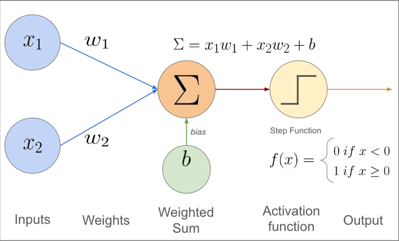
A perceptron receives inputs x₁, x₂, ..., xₙ and multiplies each by a corresponding weight w₁, w₂, ..., wₙ.

The weights represent how important each input is. If a weight is large, that input matters more in the final decision.

Mathematically, we compute a weighted sum:

z = w₁x₁ + w₂x₂ + ... + wₙxₙ + b

Here, b is the bias—it shifts the decision threshold, controlling when the perceptron fires. In our course-passing analogy, it's related to the 50-point threshold that determines whether a person passes the course. The bias allows the perceptron to make decisions even when all inputs are zero and gives it flexibility in where it draws the decision boundary.

This is a mathematical equation applied to the weighted sum of a neuron's inputs (and its bias) to determine its output signal. It acts as a "gatekeeper" or "switch" that decides whether a neuron should be "activated" (fire) and to what degree that signal should be passed to the next layer in a neural network.

Once we have the weighted sum z, we feed it into an activation function f(z), which determines the output.

For a classic perceptron, a common activation function is the step function:

f(z) = 1 if z ≥ 0, otherwise f(z) = 0

Or alternatively:

f(z) = 1 if z ≥ 0, otherwise f(z) = -1

This produces a binary output: the perceptron either fires (output = 1) or doesn't fire (output = 0 or -1).

In the resume screening scenario:

• Inputs: Each factor on the resume (experience score, skills score, motivation/cultural fit score)
• Weights: The importance you assign to each factor—how much it influences your decision
• Bias: Your personal hiring standard, the threshold that determines whether the summed score is enough to trigger a positive decision
• Weighted sum: The total score after weighing all factors
• Activation function: The yes/no hiring decision
• Learning: Adjusting how much you weigh each factor after seeing the outcomes of past hires

In the student evaluation scenario:

• Inputs: Student percentages for coursework and main exam
• Weights: How much each component counts toward the final decision
• Bias: Related to the minimum final score required to pass
• Weighted sum: The final combined score
• Activation function/Output: Pass or fail
• Learning: Adjusting weights if the outcomes don't match expectations or proven student success patterns

The power of a perceptron lies not just in making decisions, but in learning from mistakes. The perceptron learning algorithm works as follows:

1. Initialize: Start with random weights and bias
2. Predict: For each training example, calculate the weighted sum and apply the activation function to make a prediction
3. Compare: Check if the prediction matches the actual label (the correct answer)
4. Update: If there's an error, adjust the weights and bias to reduce that error
5. Repeat: Continue this process over many examples until the perceptron makes few or no errors

The weight update rule is straightforward: if the perceptron predicts 0 when it should predict 1, increase the weights for inputs that were active (non-zero). If it predicts 1 when it should predict 0, decrease those weights. The magnitude of the adjustment is controlled by a learning rate parameter.

Through this iterative process, the perceptron gradually learns the decision boundary that best separates the two classes in the training data.

We know that a perceptron is like a careful hiring manager, learning over time which factors truly matter. And just like a team of experienced hiring managers working together can make far better decisions than a single one, networks of perceptrons (neural networks), stacked and connected in layers, can tackle far more complex problems than an individual perceptron could.

A single perceptron can only learn to separate data that is linearly separable—meaning it can draw a straight line (or hyperplane in higher dimensions) to divide two classes. But by combining multiple perceptrons in layers, neural networks can learn complex, non-linear decision boundaries and solve problems that would be impossible for a single perceptron.

While perceptrons are foundational, they do have limitations:

• Linear separability constraint: A single perceptron can only solve problems where the classes can be separated by a straight line. It famously cannot solve the XOR problem, where the relationship between inputs and outputs is non-linear.
• Binary classification only: Standard perceptrons are limited to two-class problems, though this can be extended with multiple perceptrons.
• Sensitivity to feature scaling: Inputs on different scales can cause some weights to dominate others, affecting learning efficiency.
• No probabilistic output: Unlike modern activation functions (like sigmoid or softmax), the step function provides no measure of confidence—just a hard yes or no.

These limitations motivated the development of multi-layer perceptrons (MLPs) and modern neural networks, which overcome these constraints by stacking multiple layers of neurons with non-linear activation functions.

The perceptron remains a cornerstone concept in machine learning and neural networks. Understanding how it takes inputs, weighs them, sums them, and makes binary decisions through an activation function provides the foundation for understanding more complex architectures. Whether you're evaluating resumes, grading students, or building sophisticated AI systems, the core principle remains the same: learn from examples, adjust your decision-making criteria, and improve over time.